02. Estimating TTC with Lidar
Estimating TTC with Lidar
ND313 C03 L02 A02 C22 Intro
The Math Behind Time-to-Collision (TTC)
In the following, let us assume that our CAS-equipped vehicle is using a Lidar sensor to take distance measurements on preceding vehicles. The sensor in this scenario will give us the distance to the closest 3D point in the path of driving. In the figure below, the closest point is indicated by a red line emanating from a Lidar sensor on top of the CAS vehicle.
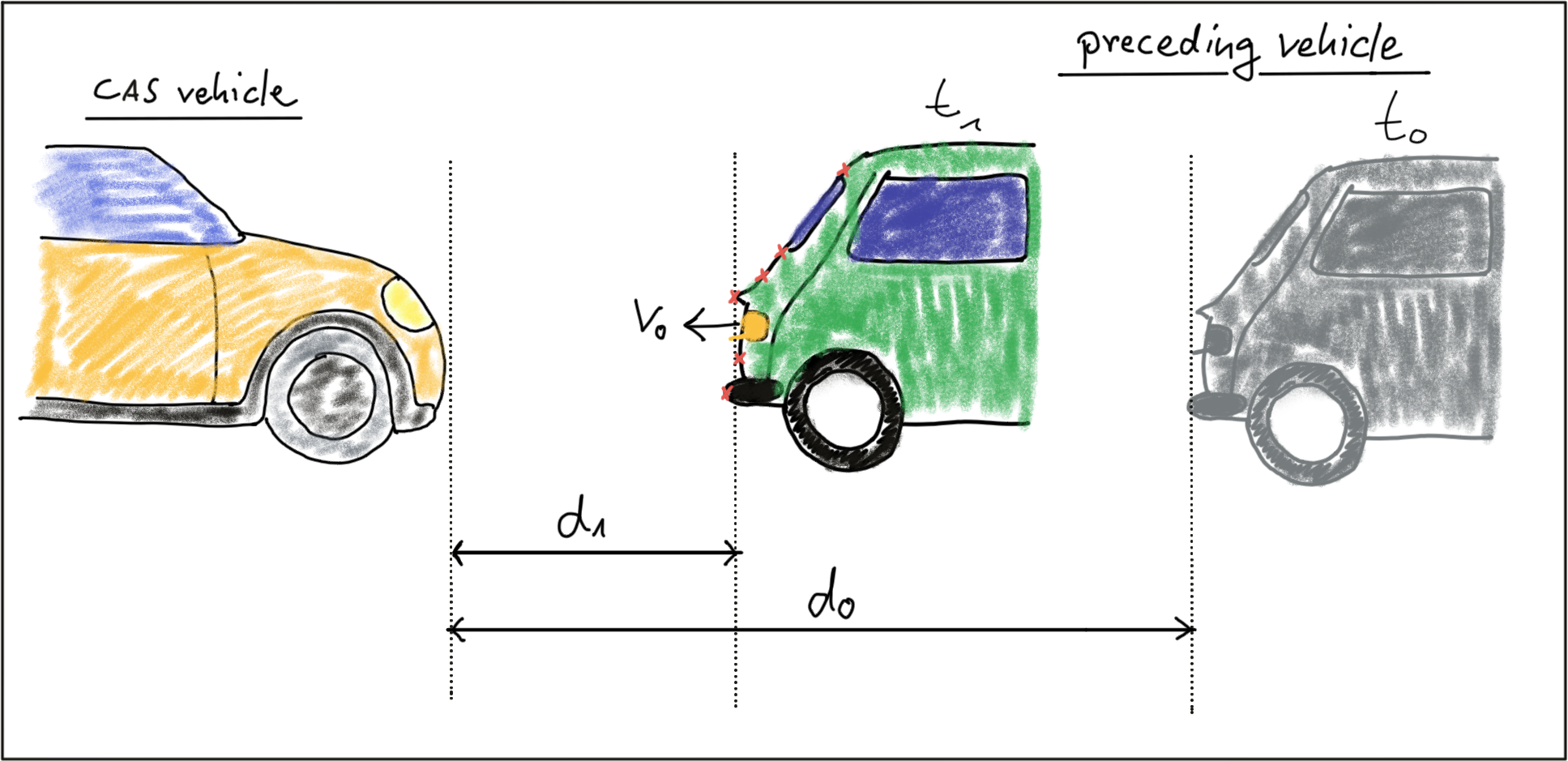
Based on the model of a constant-velocity we discussed in the last section, the velocity v_0 can be computed from two successive Lidar measurements as follows:
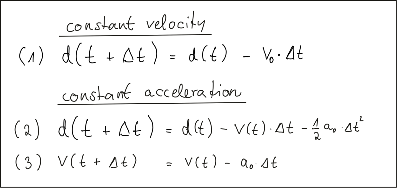
Once the relative velocity v_0 is known, the time to collision can easily be computed by dividing the remaining distance between both vehicles by v_0 . So given a Lidar sensor which is able to take precise distance measurements, a system for TTC estimation can be developed based based on a CVM and on the set of equations shown above. Note however that a radar sensor would be the superior solution for TTC computation as it can directly measure the relative speed, whereas with the Lidar sensor we need to compute v_0 from two (noisy) distance measurements.
Preparing the Lidar Point Cloud
The following image shows a Lidar point cloud as an overlay over a camera image taken in a highway scenario with a preceding vehicle directly in the path of driving. Distance to the sensor is color-coded (green is far away, red is close). On the left side, a bird-view perspective of the Lidar points is shown as well.
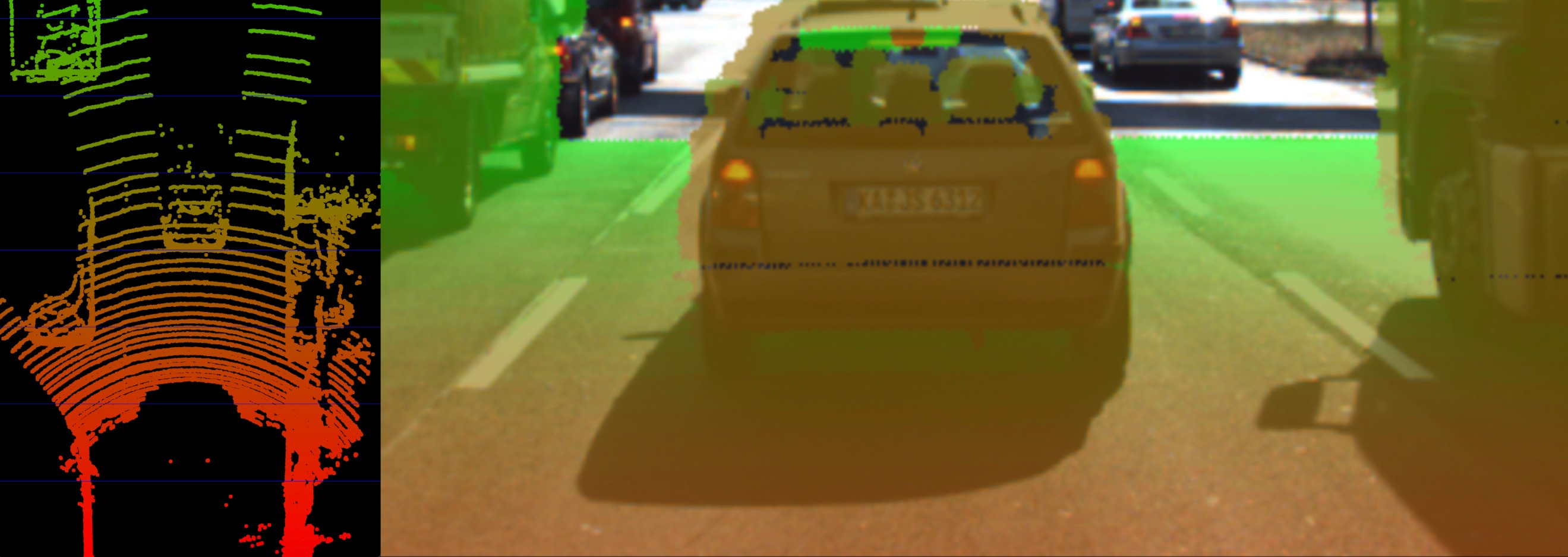
As can easily be seen, the Lidar sensor provides measurements on the vehicles as well as on the road surface. Also, some 3D points in the camera image do not seem accurate when compared to their surrounding neighbors. Especially the points near the roof of the preceding vehicle differ in color from the points on the tailgate.
As measurement accuracy is correlated to the amount of light reflected from an object, it makes sense to consider the reflectiveness r of each Lidar point which we can access in addition to the x, y and z coordinates. The image below highlights high reflectiveness with green, whereas regions with low reflectiveness are shown as red. An analysis of the associated reflectivity of the point cloud shows that such deviations often occur in regions with reduced reflectiveness.
In order to derive a stable TTC measurement from the given point cloud, two main steps have to be performed:
- Remove measurements on the road surface
- Remove measurements with low reflectivity
In the figure below, Lidar points are shown in a top-view perspective and as an image overlay after applying the filtering. After removing Lidar points in this manner, it is now much easier to derive the distance d(t) to the preceding vehicle.
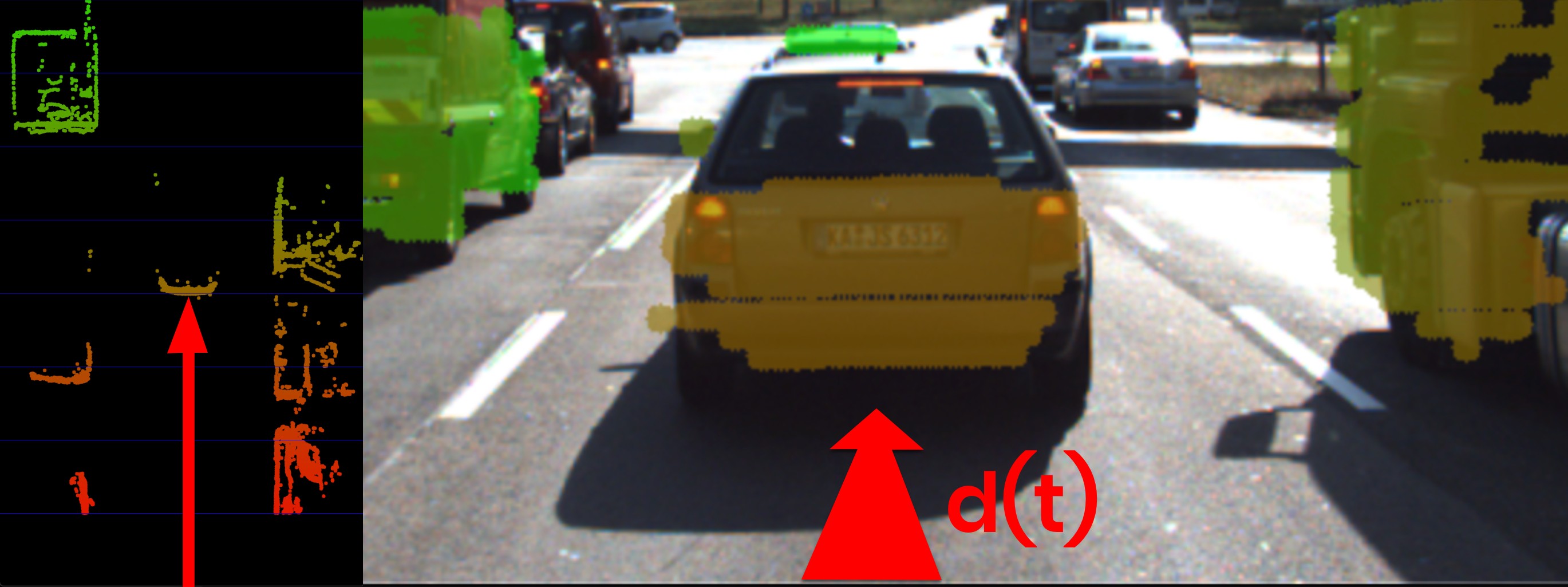
In a later lesson, you will learn how to project Lidar points into the camera image and how to perform the removal procedure as seen in the above examples. For now, let us assume that for each time step dt, the Lidar sensor would return the distance d(t+dt) to the preceding vehicle.
Computing TTC from Distance Measurements
In the code examples in this course, Lidar points are packaged into a data structure called LidarPoints. As seen below, the structure consists of the point coordinates x (forward), y (left) an z (up) in metric coordinates and of the point reflectivity r on a scale between 0 and 1 (high reflectivity).
struct LidarPoint { // single lidar point in space
double x, y, z; // point position in m
double r; // point reflectivity in the range 0-1
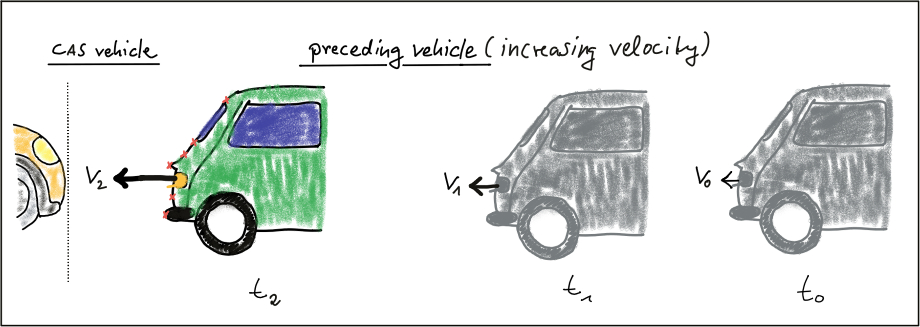
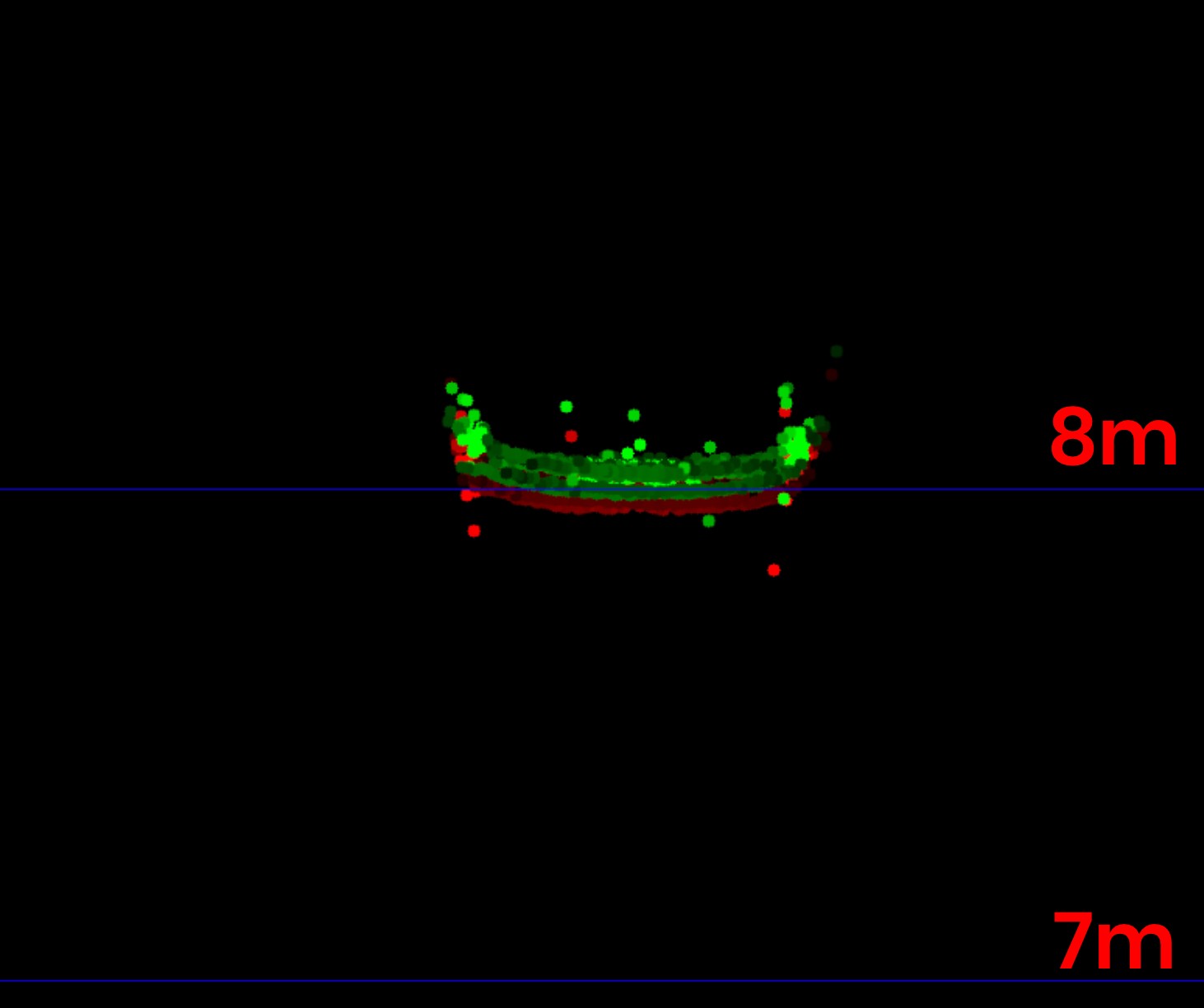
};In order to compute the TTC, we need to find the distance to the closest Lidar point in the path of driving. In the figure below, Lidar measurements located on the tailgate of the preceding vehicle are measured at times t_0 (green) and t_1 (red). It can be seen, that the distance to the vehicle has decreased slightly between both time instants.
The following code searches for the closest point in the point cloud associated with
t_0
(
lidarPointsPrev
) and in the point cloud associated with
t_1
(
lidarPointsCurr
). After finding the distance to the closest points respectively, the TTC is computed based on the formula we derived at the beginning of this section.
void computeTTCLidar(std::vector<LidarPoint> &lidarPointsPrev,
                     std::vector<LidarPoint> &lidarPointsCurr, double &TTC)
{
    // auxiliary variables
    double dT = 0.1; // time between two measurements in seconds

    // find closest distance to Lidar points
    double minXPrev = 1e9, minXCurr = 1e9;
    for(auto it=lidarPointsPrev.begin(); it!=lidarPointsPrev.end(); ++it) {
        minXPrev = minXPrev>it->x ? it->x : minXPrev;
    }

    for(auto it=lidarPointsCurr.begin(); it!=lidarPointsCurr.end(); ++it) {
        minXCurr = minXCurr>it->x ? it->x : minXCurr;
    }

    // compute TTC from both measurements
    TTC = minXCurr * dT / (minXPrev-minXCurr);
}
Even though Lidar is a reliable sensor, erroneous measurements may still occur. As seen in the figure above, a small number of points is located behind the tailgate, seemingly without connection to the vehicle. When searching for the closest points, such measurements will pose a problem as the estimated distance will be too small. There are ways to avoid such errors by post-processing the point cloud, but there will be no guarantee that such problems will never occur in practice. It is thus a good idea to perform a more robust computation of minXCurr and minXPrev which is able to cope with a certain number of outliers (in the final project, you will do this) and also look at a second sensor which is able to compute the TTC, such as the camera.
Exercise
ND313 C03 L02 A03 C22 Quiz
In the workspace below, extend the function
computeTTCLidar
shown above so that only Lidar points within a narrow corridor whose width is defined by a variable laneWidth are considered during minimum search. The width of the corridor should be set to 4 meters.
You can run your code as usual by creating a
build
directory in
TTC_lidar
. Then use the following steps from within the
build
directory:
-
cmake .. -
make -
./compute_ttc_lidar
Workspace
This section contains either a workspace (it can be a Jupyter Notebook workspace or an online code editor work space, etc.) and it cannot be automatically downloaded to be generated here. Please access the classroom with your account and manually download the workspace to your local machine. Note that for some courses, Udacity upload the workspace files onto https://github.com/udacity , so you may be able to download them there.
Workspace Information:
- Default file path:
- Workspace type: react
- Opened files (when workspace is loaded): n/a
-
userCode:
             export CXX=g++-7


              export CXXFLAGS=-std=c++17